hdmax2 helper functions
Florence Pittion, Magali Richard, Olivier Francois
January, 2024
helper_functions.RmdIntroduction
The hdmax2 package is designed to accept exposure \(X\) consisting of univariate data, which
can be continuous, binary, or categorical, as well as multivariate
exposomes. Binary variables are converted to 0s and 1s and treated as
univariate variables.
In this vignette, we provide a series of helper function to process the data.
To install the latest version of hdmax2, use the github
repository
#devtools::install_github("bcm-uga/hdmax2")How to analyse agregated methylated regions ?
We simulated 500 samples and 1000 potential DNA methylation mediators, with various a binary exposure (smoking status of mothers) and continuous outcomes (birth weight).
Identifying aggregated mediator regions (AMR)
Identify Aggregated Methylated regions (AMR) with AMR_search function
which uses from the P-values from max-squared test compute in
run_AS function and using a adapted comb-p method (comb-p
is a tool that manipulates BED files of possibly irregularly spaced
P-values and calculates auto-correlation, combines adjacent P-values,
performs false discovery adjustment, finds regions of enrichment and
assigns significance to those regions). AMR identification could be
useful in Epigenomic Wide Association Studies when single CpG mediation
is unsuccessful, or could be complementary analysis.
data = hdmax2::helper_ex

#Artificial reduction of dataset size to pass the github action check when building hdmax2 website
data$methylation = data$methylation[ , 800:1000]
data$annotation = data$annotation[800:1000, ]


pc <- prcomp(data$methylation)
plot((pc$sdev^2/sum(pc$sdev^2))[1:15],
     xlab = 'Principal Component',
     ylab = "Explained variance",
     col = c(rep(1, 3), 2, rep(1, 16)))
# chosen number of dimension
K=5

## run hdmax2 step1
hdmax2_step1 = hdmax2::run_AS(X = data$exposure,
                              Y = data$phenotype,
                              M = data$methylation,
                              K = K)

##Detecting AMR
seed = 0.6 #Careful to change this parameter when working with real data
res.amr_search = hdmax2::AMR_search(chr = data$annotation$chr,
                                    start = data$annotation$start,
                                    end = data$annotation$end,
                                    pval = hdmax2_step1$max2_pvalues,
                                    cpg = data$annotation$cpg,
                                    seed = seed,
                                    nCores = 2)

res.amr_search$res
#>   chr   start     end           p        fdr
#> 2   1 1326166 1326221 0.005626678 0.01688003
#> 1   1 1310734 1310988 0.019799860 0.02138751
#> 3   1 1406862 1407016 0.021387509 0.02138751

res.arm_build = hdmax2::AMR_build(res.amr_search,
                                  methylation = data$methylation,
                                  nb_cpg = 2)

#List of DMR selected
head(res.arm_build$res)
#>    DMR chr   start     end          p        fdr nb
#> 1 DMR1   1 1310734 1310988 0.01979986 0.02138751  2
#> 2 DMR2   1 1406862 1407016 0.02138751 0.02138751  2

##CpG in the DMR
res.arm_build$CpG_for_each_AMR
#> $DMR1
#> [1] "cg11518257" "cg15617543"
#>
#> $DMR2
#> [1] "cg10228629" "cg06377929"
Quantifying indirect effects
Like with single mediators analysis esimate_effect function
could be use to estimate different effects of AMR. Also
plot_hdmax2 can be applied to step2 results.
## run hdmax2 step2
object = hdmax2_step1
mediators_top10 = data$methylation[,names(sort(hdmax2_step1$max2_pvalues)[1:10])]
m = as.matrix(res.arm_build$AMR_mean)
boots = 100
## selected mediators effects estimation

hdmax2_step2 = hdmax2::estimate_effect(object = hdmax2_step1,
                                       m = m,
                                       boots = 100)
library(ggplot2)
hdmax2::plot_hdmax2(hdmax2_step2, plot_type= "all_plot")
#> [1] "hdmax2 plot for univariate exposome"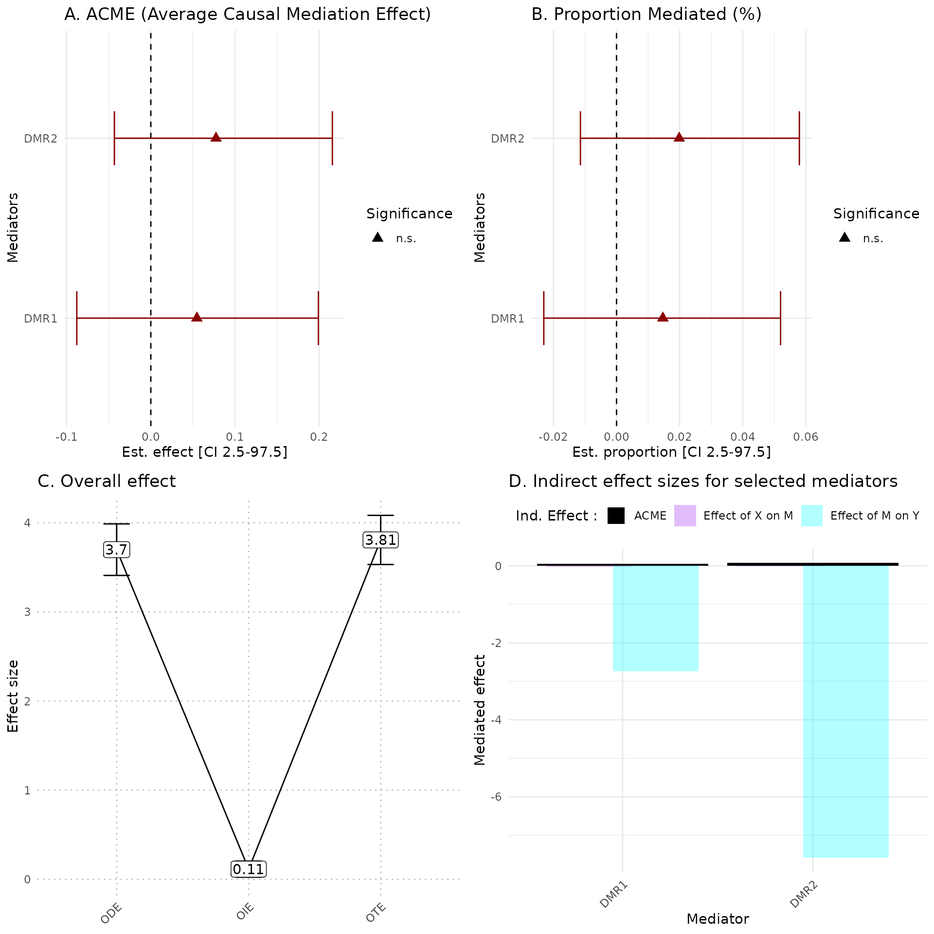
#> TableGrob (2 x 2) "arrange": 4 grobs
#>   z     cells    name           grob
#> 1 1 (1-1,1-1) arrange gtable[layout]
#> 2 2 (1-1,2-2) arrange gtable[layout]
#> 3 3 (2-2,1-1) arrange gtable[layout]
#> 4 4 (2-2,2-2) arrange gtable[layout]
How to select potential mediators using q-values and FDR control ?
Several methods can be use to select potential mediators from step1
results of our method, in our main use cases we simply select top 10
mediators to simplify the narrative. Among available methods to select
mediators from mediation test p-values, we can use FDR (False Discovery
Rate) control. Q-value is obtained from max-squared test
p-values from step 1 with fdrtools::fdrtools function then
bounded by chosen threshold.
data_sim = hdmax2::simu_data
## run hdmax2 step1
hdmax2_step1 = hdmax2::run_AS(X = data_sim$X_binary,
                 Y = data_sim$Y_continuous,
                 M = data_sim$M1,
                 K = K)

## Select candidate mediator
qval <- fdrtool::fdrtool(hdmax2_step1$max2_pvalues, statistic = "pvalue", plot = F, verbose = F)$qval
candidate_mediator <- qval[qval<= 0.2] # In this example, we will consider FDR levels <20%.
candidate_mediator
#>   cg00018896   cg00019093   cg00022633   cg00024247   cg00025981   cg00028749
#> 1.107337e-02 3.873482e-10 3.409990e-15 3.174703e-02 4.013016e-06 3.457313e-02
#>   cg00031759   cg00035636   cg00037930   cg00047079   cg00049102   cg00049382
#> 1.076710e-04 2.157911e-08 1.176850e-01 2.609498e-02 8.673316e-09 2.705899e-04
#>   cg00049616   cg00241432   cg00345862   cg01005425
#> 2.419102e-05 1.952512e-01 9.383553e-02 1.688914e-01
How to transform a categorial variable into an ordered factor?
When categorical variables are used as exposure variables,
hdmax2 uses the first category as a reference (intercept)
to calculate the effects associated with the variable’s other
categories. The functions HDMAX2::run_AS and
HDMAX2::estimate_effect will transform the character vector
you have used (if any) into a factor, with an arbitrary ordering of the
categories. If order is important to you, here’s a simple way to turn
your character vector into a factor and order the categories as you
wish. You can then use this variable as input to the hdmax2
functions.
How to handle adding an additional set of covariates to the second association study?
It is possible to add a second adjustment factors set in association study between potential mediators and outcome if it makes sense from a biological standpoint. Nevertheless, this additional set of adjustment factors for the second association study must include the adjustment factors from the first association study.
covar = as.data.frame(data$covariables[,1:2])
covar_sup_reg2 = as.data.frame(data$covariables[,3:4])

hdmax2_step1 = hdmax2::run_AS(X = data$exposure,
                              Y = data$phenotype,
                              M = data$methylation,
                              K = K,
                              covar = covar,
                              covar_sup_reg2 = covar_sup_reg2)
sessionInfo()
#> R version 4.3.3 (2024-02-29)
#> Platform: x86_64-pc-linux-gnu (64-bit)
#> Running under: Ubuntu 22.04.4 LTS
#>
#> Matrix products: default
#> BLAS:   /usr/lib/x86_64-linux-gnu/openblas-pthread/libblas.so.3
#> LAPACK: /usr/lib/x86_64-linux-gnu/openblas-pthread/libopenblasp-r0.3.20.so;  LAPACK version 3.10.0
#>
#> locale:
#>  [1] LC_CTYPE=C.UTF-8       LC_NUMERIC=C           LC_TIME=C.UTF-8
#>  [4] LC_COLLATE=C.UTF-8     LC_MONETARY=C.UTF-8    LC_MESSAGES=C.UTF-8
#>  [7] LC_PAPER=C.UTF-8       LC_NAME=C              LC_ADDRESS=C
#> [10] LC_TELEPHONE=C         LC_MEASUREMENT=C.UTF-8 LC_IDENTIFICATION=C
#>
#> time zone: UTC
#> tzcode source: system (glibc)
#>
#> attached base packages:
#> [1] stats     graphics  grDevices utils     datasets  methods   base
#>
#> other attached packages:
#> [1] ggplot2_3.5.0
#>
#> loaded via a namespace (and not attached):
#>  [1] tidyselect_1.2.1        farver_2.1.1            dplyr_1.1.4
#>  [4] Biostrings_2.70.3       bitops_1.0-7            fastmap_1.1.1
#>  [7] RCurl_1.98-1.14         digest_0.6.35           rpart_4.1.23
#> [10] lifecycle_1.0.4         cluster_2.1.6           magrittr_2.0.3
#> [13] compiler_4.3.3          rlang_1.1.3             Hmisc_5.1-2
#> [16] sass_0.4.9              tools_4.3.3             utf8_1.2.4
#> [19] yaml_2.3.8              data.table_1.15.4       knitr_1.45
#> [22] labeling_0.4.3          htmlwidgets_1.6.4       mediation_4.5.0
#> [25] foreign_0.8-86          withr_3.0.0             purrr_1.0.2
#> [28] BiocGenerics_0.48.1     desc_1.4.3              nnet_7.3-19
#> [31] grid_4.3.3              stats4_4.3.3            fansi_1.0.6
#> [34] colorspace_2.1-0        scales_1.3.0            MASS_7.3-60.0.1
#> [37] cli_3.6.2               mvtnorm_1.2-4           rmarkdown_2.26
#> [40] crayon_1.5.2            ragg_1.3.0              generics_0.1.3
#> [43] rstudioapi_0.16.0       minqa_1.2.6             cachem_1.0.8
#> [46] stringr_1.5.1           zlibbioc_1.48.2         splines_4.3.3
#> [49] parallel_4.3.3          XVector_0.42.0          base64enc_0.1-3
#> [52] vctrs_0.6.5             boot_1.3-29             Matrix_1.6-5
#> [55] sandwich_3.1-0          jsonlite_1.8.8          IRanges_2.36.0
#> [58] S4Vectors_0.40.2        Formula_1.2-5           htmlTable_2.4.2
#> [61] systemfonts_1.0.6       jquerylib_0.1.4         glue_1.7.0
#> [64] pkgdown_2.0.7           nloptr_2.0.3            stringi_1.8.3
#> [67] gtable_0.3.4            GenomeInfoDb_1.38.8     hdmax2_2.0.0.9000
#> [70] lme4_1.1-35.2           munsell_0.5.1           tibble_3.2.1
#> [73] pillar_1.9.0            htmltools_0.5.8         GenomeInfoDbData_1.2.11
#> [76] R6_2.5.1                textshaping_0.3.7       evaluate_0.23
#> [79] lpSolve_5.6.20          lattice_0.22-5          highr_0.10
#> [82] backports_1.4.1         memoise_2.0.1           bslib_0.7.0
#> [85] fdrtool_1.2.17          Rcpp_1.0.12             gridExtra_2.3
#> [88] nlme_3.1-164            checkmate_2.3.1         xfun_0.43
#> [91] fs_1.6.3                zoo_1.8-12              prettydoc_0.4.1
#> [94] pkgconfig_2.0.3