Predict polygenic scores from latent factor models

This function computes polygenic risk scores from the estimates of latent factor models. It uses the indirect' effect sizes for the regression of X (a single phenotype) on the matrix Y, for predicting phenotypic values for new genotype data.

predict_lfmm(Y, X, lfmm.object, fdr.level = 0.1, newdata = NULL)

Arguments

Y	a response variable matrix with n rows and p columns, typically containing genotypes. Each column is a response variable (numeric).
X	an explanatory variable with n rows and d = 1 column (numeric) representing a phenotype with zero mean across the sample.
lfmm.object	an object of class lfmm returned by the lfmm_lasso or lfmm_ridge function, computed for X and Y.
fdr.level	a numeric value for the FDR level in the lfmm test used to define candidate variables for predicting new phenotypes.
newdata	a matrix with n rows and p' columns, and similar to Y, on which predictions of X will be based. If NULL, Y is used as new data.

Value

a list with the following attributes:

• prediction: a vector of length n containing the predicted values for X. If newdata = NULL, the fitted values are returned.

• candidates: a vector of candidate columns of Y on which the predictions are built.

Details

The response variable matrix Y and the explanatory variable are centered.

Examples

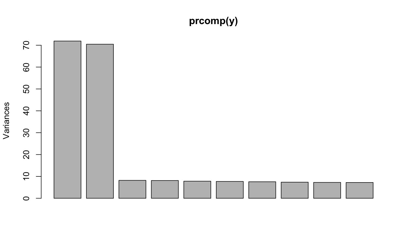
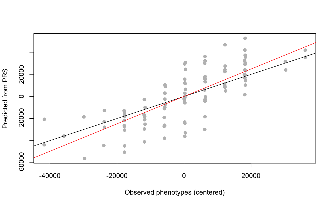
library(lfmm)

## Simulation of 1000 genotypes for 100 individuals (y)
u <- matrix(rnorm(300, sd = 1), nrow = 100, ncol = 2)
v <- matrix(rnorm(3000, sd = 2), nrow = 2, ncol = 1000)
y <- matrix(rbinom(100000, size = 2,
                  prob = 1/(1 + exp(-0.3*(u%*%v
                  + rnorm(100000, sd = 2))))),
                  nrow = 100,
                  ncol = 1000)

#PCA of genotypes, 2 main axes of variation (K = 2) 
plot(prcomp(y))

## Simulation of 1000 phenotypes (x)
## Only the last 10 genotypes have significant effect sizes (b)
b <- matrix(c(rep(0, 990), rep(6000, 10)))
x <- y%*%b + rnorm(100, sd = 100)

## Compute effect sizes using lfmm_ridge
mod <- lfmm_ridge(Y = y,
                  X = x,
                  K = 2)

x.pred <- predict_lfmm(Y = y,
                       X = x,
                       fdr.level = 0.25,
                       mod)

x.pred$candidates
#> [1] 999 996 994 998 820 127 444 421 997

##Compare simulated and predicted/fitted phenotypes
plot(x - mean(x), x.pred$pred,
     pch = 19, col = "grey",
     xlab = "Observed phenotypes (centered)",
     ylab = "Predicted from PRS")
abline(0,1)
abline(lm(x.pred$pred ~ scale(x, scale = FALSE)), col = 2)