LFMM least-squares estimates with ridge penalty

This function computes regularized least squares estimates for latent factor mixed models using a ridge penalty.

lfmm_ridge(Y, X, K, lambda = 1e-05, algorithm = c("analytical",
  "alternated"), it.max = 100, relative.err.min = 1e-06)

Arguments

Y	a response variable matrix with n rows and p columns. Each column corresponds to a distinct response variable (e.g., SNP genotype, gene expression level, beta-normalized methylation profile, etc). Response variables must be encoded as numeric.
X	an explanatory variable matrix with n rows and d columns. Each column corresponds to a distinct explanatory variable (eg. phenotype). Explanatory variables must be encoded as numeric variables.
K	an integer for the number of latent factors in the regression model.
lambda	a numeric value for the regularization parameter.
algorithm	analytical solution algorithm or numerical alternated algorithm. The analytical solution algorithm is based on global minimum of the loss function and the computation is very quick. The numerical alternated algorithm converges toward a local minimum of the loss function. The interest of the alternated algorithm is that it does not imply the computation of a \(n \times n\) matrix. Whereas the analytical algorithm requires the computation of a \(n \times n\) matrix, which can be a problem when n is very large.
it.max	an integer value for the number of iterations of the algorithm. Only for the alternated numerical algorithm
relative.err.epsilon	a numeric value for a relative convergence error. Determine whether the algorithm converges or not. Only for the alternated numerical algorithm.

Value

an object of class lfmm with the following attributes:

• U the latent variable score matrix with dimensions n x K,

• V the latent variable axis matrix with dimensions p x K,

• B the effect size matrix with dimensions p x d.

Details

The algorithm minimizes the following penalized least-squares criterion $$ L(U, V, B) = \frac{1}{2} ||Y - U V^{T} - X B^T||_{F}^2 + \frac{\lambda}{2} ||B||^{2}_{2} ,$$ where Y is a response data matrix, X contains all explanatory variables, U denotes the score matrix, V is the loading matrix, B is the (direct) effect size matrix, and lambda is a regularization parameter.

The response variable matrix Y and the explanatory variable are centered.

Examples

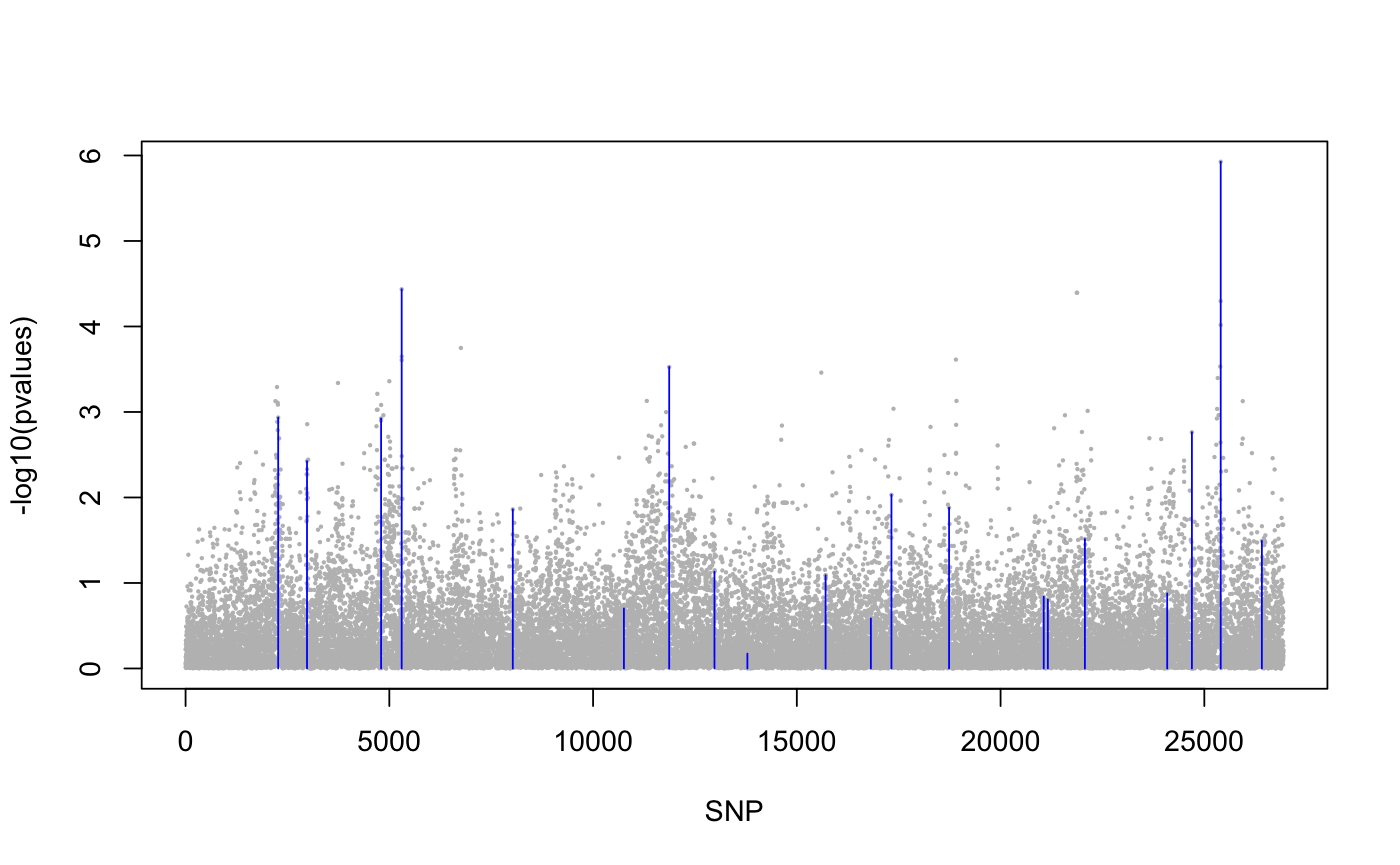
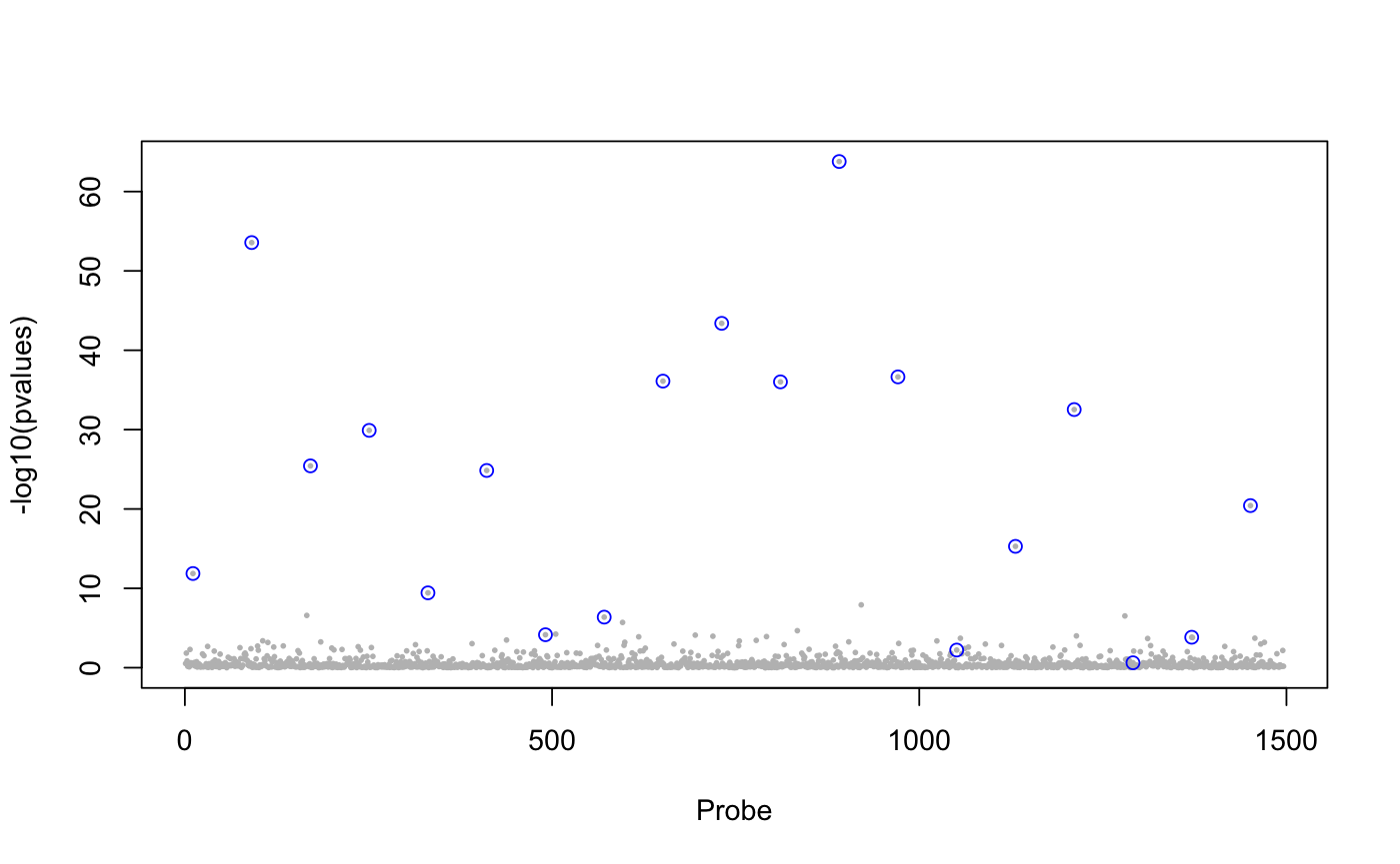
library(lfmm)

## a GWAS example with Y = SNPs and X = phenotype
data(example.data)
Y <- example.data$genotype
X <- example.data$phenotype

## Fit an LFMM with K = 6 factors
mod.lfmm <- lfmm_ridge(Y = Y,
                       X = X,
                       K = 6)

## Perform association testing using the fitted model:
pv <- lfmm_test(Y = Y,
                X = X,
                lfmm = mod.lfmm,
                calibrate = "gif")

## Manhattan plot with causal loci shown

pvalues <- pv$calibrated.pvalue
plot(-log10(pvalues), pch = 19,
     cex = .2, col = "grey", xlab = "SNP")
points(example.data$causal.set,
      -log10(pvalues)[example.data$causal.set],
       type = "h", col = "blue")


## An EWAS example with Y = methylation data and X = exposure
Y <- scale(skin.exposure$beta.value)
X <- scale(as.numeric(skin.exposure$exposure))

## Fit an LFMM with 2 latent factors
mod.lfmm <- lfmm_ridge(Y = Y,
                       X = X,
                       K = 2)

## Perform association testing using the fitted model:
pv <- lfmm_test(Y = Y,
                X = X,
                lfmm = mod.lfmm,
                calibrate = "gif")

## Manhattan plot with true associations shown
pvalues <- pv$calibrated.pvalue
plot(-log10(pvalues),
     pch = 19,
     cex = .3,
     xlab = "Probe",
     col = "grey")

causal.set <- seq(11, 1496, by = 80)
points(causal.set,
      -log10(pvalues)[causal.set],
       col = "blue")