Statistical tests with latent factor mixed models

This function returns significance values for the association between each column of the response matrix, Y, and the explanatory variables, X, including correction for unobserved confounders (latent factors). The test is based on an LFMM fitted with a ridge or lasso penalty.

lfmm_test(Y, X, lfmm, calibrate = "gif")

Arguments

Y	a response variable matrix with n rows and p columns. Each column is a response variable (numeric).
X	an explanatory variable matrix with n rows and d columns. Each column corresponds to an explanatory variable (numeric).
lfmm	an object of class lfmm returned by the lfmm_lasso or lfmm_ridge function
calibrate	a character string, "gif" or "median+MAD". If the "gif" option is set (default), significance values are calibrated by using the genomic control method. Genomic control uses a robust estimate of the variance of z-scores called "genomic inflation factor". If the "median+MAD" option is set, the pvalues are calibrated by computing the median and MAD of the zscores. If NULL, the pvalues are not calibrated.

Value

a list with the following attributes:

• B the effect size matrix with dimensions p x d.

• score a p x d matrix which contains z-scores for each explanatory variable (columns of X),

• pvalue a p x d matrix which contains p-values for each explanatory variable,

• calibrated.pvalue a p x d matrix which contains calibrated p-values for each explanatory variable,

• gif a numeric value for the genomic inflation factor.

Details

The response variable matrix Y and the explanatory variable are centered.

Examples

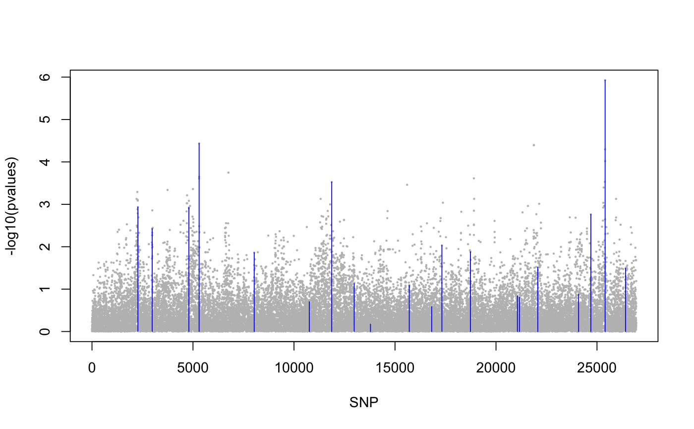
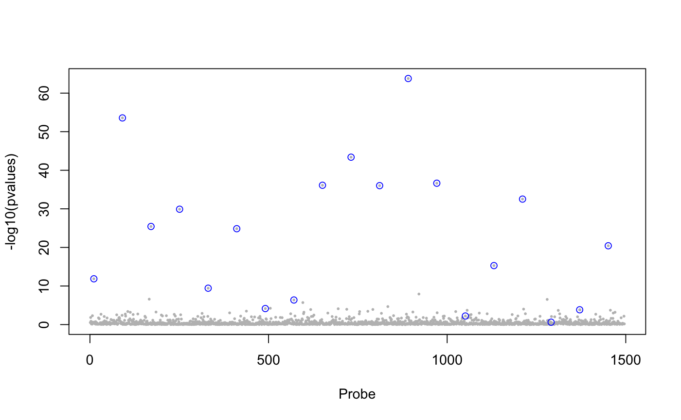
library(lfmm)

## a GWAS example with Y = SNPs and X = phenotype
data(example.data)
Y <- example.data$genotype
X <- example.data$phenotype

## Fit an LFMM with K = 6 factors
mod.lfmm <- lfmm_ridge(Y = Y,
                       X = X,
                       K = 6)

## Perform association testing using the fitted model:
pv <- lfmm_test(Y = Y,
                X = X,
                lfmm = mod.lfmm,
                calibrate = "gif")

## Manhattan plot with causal loci shown

pvalues <- pv$calibrated.pvalue
plot(-log10(pvalues), pch = 19,
     cex = .2, col = "grey", xlab = "SNP")
points(example.data$causal.set,
      -log10(pvalues)[example.data$causal.set],
       type = "h", col = "blue")


## An EWAS example with Y = methylation data and X = exposure
Y <- scale(skin.exposure$beta.value)
X <- scale(as.numeric(skin.exposure$exposure))

## Fit an LFMM with 2 latent factors
mod.lfmm <- lfmm_ridge(Y = Y,
                       X = X,
                       K = 2)

## Perform association testing using the fitted model:
pv <- lfmm_test(Y = Y,
                X = X,
                lfmm = mod.lfmm,
                calibrate = "gif")

## Manhattan plot with true associations shown
pvalues <- pv$calibrated.pvalue
plot(-log10(pvalues),
     pch = 19,
     cex = .3,
     xlab = "Probe",
     col = "grey")

causal.set <- seq(11, 1496, by = 80)
points(causal.set,
      -log10(pvalues)[causal.set],
       col = "blue")