LFMM least-squares estimates with lasso penalty
This function computes regularized least squares estimates for latent factor mixed models using a lasso penalty.
lfmm_lasso(Y, X, K, nozero.prop = 0.01, lambda.num = 100,
  lambda.min.ratio = 0.01, lambda = NULL, it.max = 100,
  relative.err.epsilon = 1e-06)
Arguments
| Y | a response variable matrix with n rows and p columns. Each column is a response variable (e.g., SNP genotype, gene expression level, beta-normalized methylation profile, etc). Response variables must be encoded as numeric. |
|---|---|
| X | an explanatory variable matrix with n rows and d columns. Each column corresponds to a distinct explanatory variable (eg. phenotype). Explanatory variables must be encoded as numeric. |
| K | an integer for the number of latent factors in the regression model. |
| nozero.prop | a numeric value for the expected proportion of non-zero effect sizes. |
| lambda.num | a numeric value for the number of 'lambda' values (obscure). |
| lambda.min.ratio | (obscure parameter) a numeric value for the smallest |
| lambda | (obscure parameter) Smallest value of |
| it.max | an integer value for the number of iterations of the algorithm. |
| relative.err.epsilon | a numeric value for a relative convergence error. Determine whether the algorithm converges or not. |
Value
an object of class lfmm with the following attributes:
U the latent variable score matrix with dimensions n x K,
V the latent variable axes matrix with dimensions p x K,
B the effect size matrix with dimensions p x d.
Details
The algorithm minimizes the following penalized least-squares criterion
The response variable matrix Y and the explanatory variable are centered.
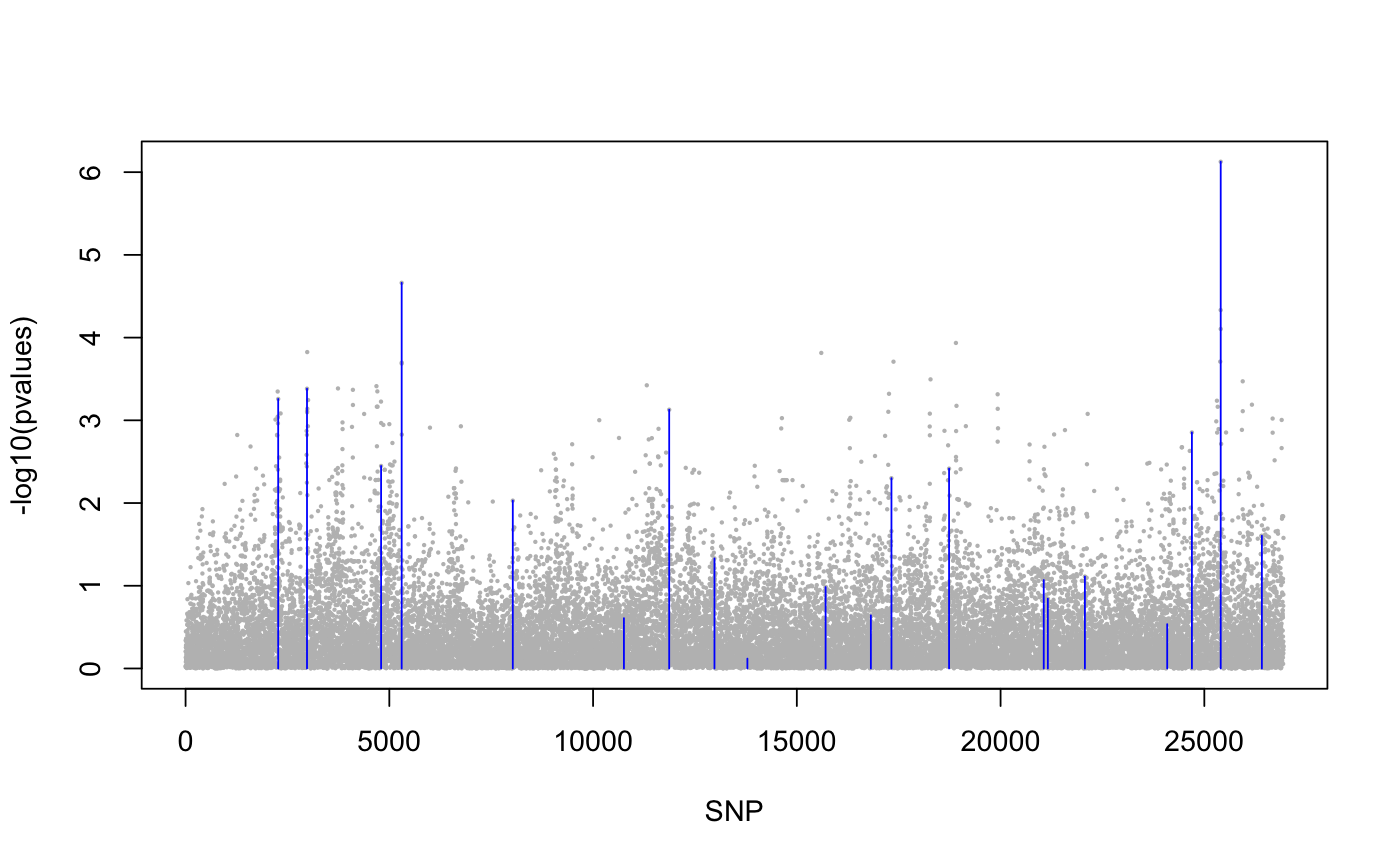
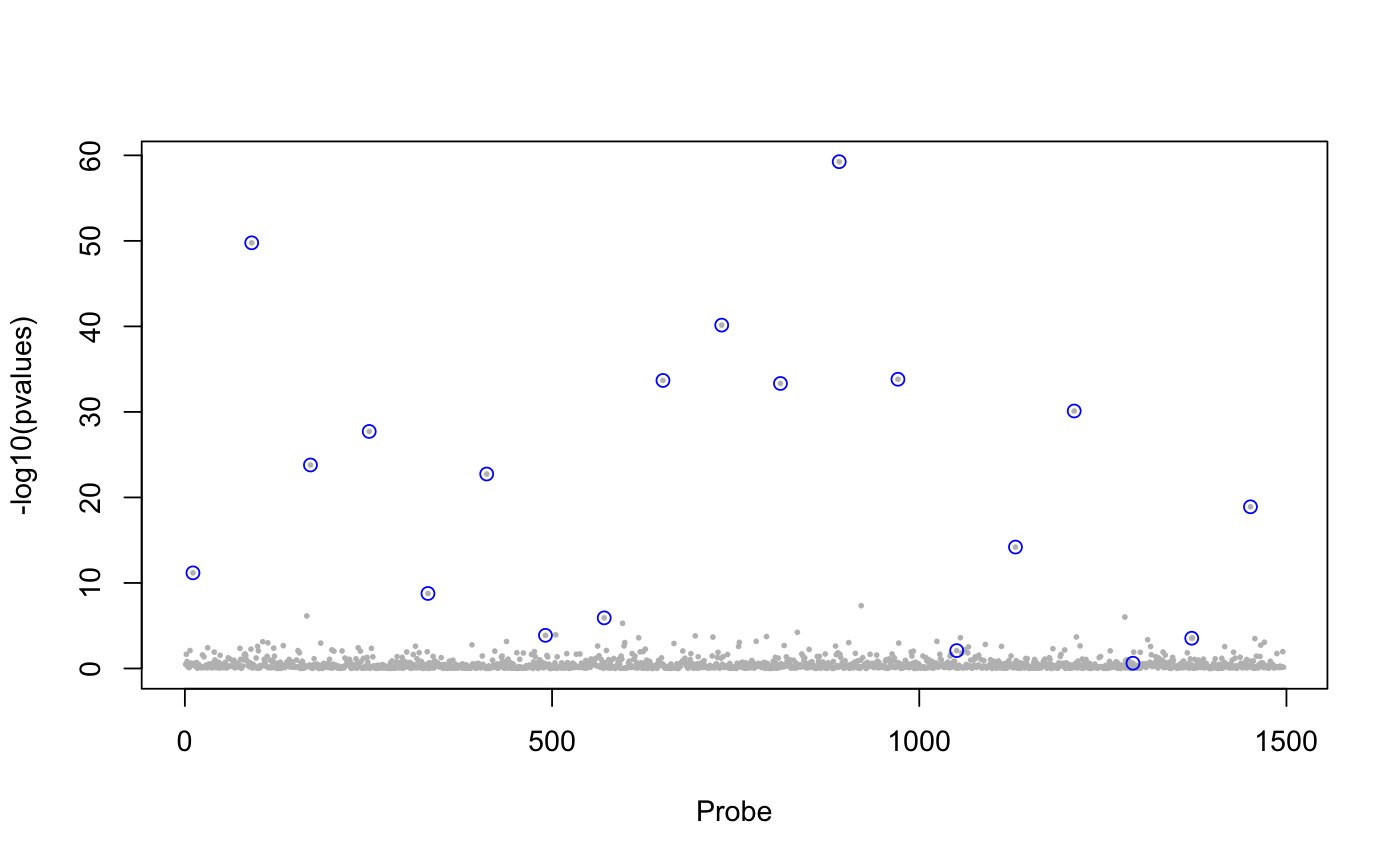
Examples
library(lfmm) ## a GWAS example with Y = SNPs and X = phenotype data(example.data) Y <- example.data$genotype X <- example.data$phenotype ## Fit an LFMM with 6 factors mod.lfmm <- lfmm_lasso(Y = Y, X = X, K = 6, nozero.prop = 0.01)#>#>#>#>#>#>#>#>#>#>#>#>#>#>#>#>#>#>#>#>#>#>#>#>#>#>#>#>#>#>## Perform association testing using the fitted model: pv <- lfmm_test(Y = Y, X = X, lfmm = mod.lfmm, calibrate = "gif") ## Manhattan plot with causal loci shown pvalues <- pv$calibrated.pvalue plot(-log10(pvalues), pch = 19, cex = .2, col = "grey", xlab = "SNP")points(example.data$causal.set, -log10(pvalues)[example.data$causal.set], type = "h", col = "blue")## An EWAS example with Y = methylation data ## and X = exposure Y <- scale(skin.exposure$beta.value) X <- scale(as.numeric(skin.exposure$exposure)) ## Fit an LFMM with 2 latent factors mod.lfmm <- lfmm_lasso(Y = Y, X = X, K = 2, nozero.prop = 0.01)#>#>#>#>#>#>#>#>## Perform association testing using the fitted model: pv <- lfmm_test(Y = Y, X = X, lfmm = mod.lfmm, calibrate = "gif") ## Manhattan plot with true associations shown pvalues <- pv$calibrated.pvalue plot(-log10(pvalues), pch = 19, cex = .3, xlab = "Probe", col = "grey")causal.set <- seq(11, 1496, by = 80) points(causal.set, -log10(pvalues)[causal.set], col = "blue")