Direct effect sizes estimated from latent factor models

This function returns 'direct' effect sizes for the regression of X (of dimension 1) on the matrix Y, as usually computed in genome-wide association studies.

effect_size(Y, X, lfmm.object)

Arguments

Y	a response variable matrix with n rows and p columns. Each column is a response variable (numeric).
X	an explanatory variable with n rows and d = 1 column (numeric).
lfmm.object	an object of class lfmm returned by the lfmm_lasso or lfmm_ridge function.

Value

a vector of length p containing all effect sizes for the regression of X on the matrix Y

Details

The response variable matrix Y and the explanatory variable are centered.

Examples

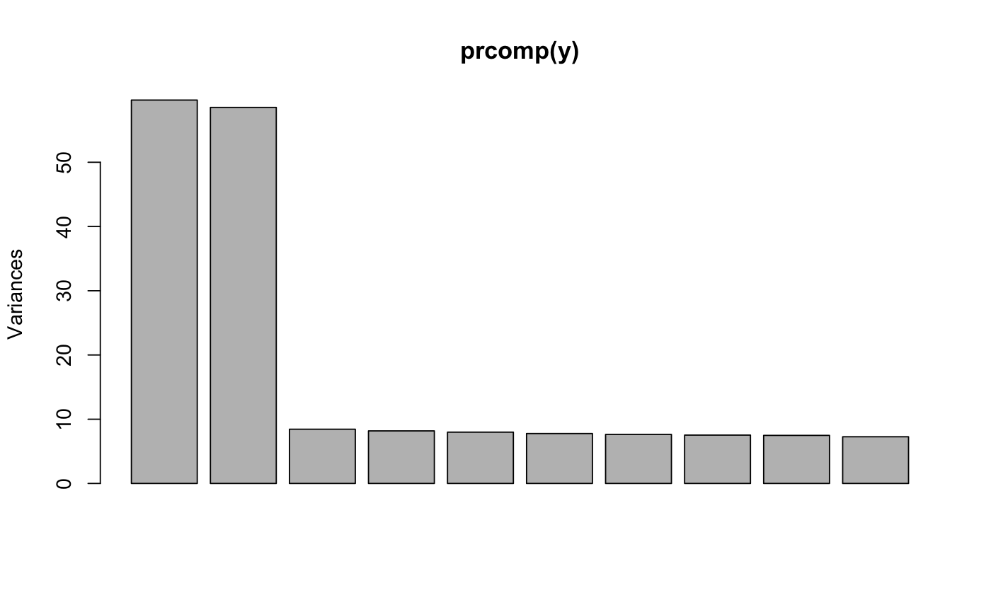
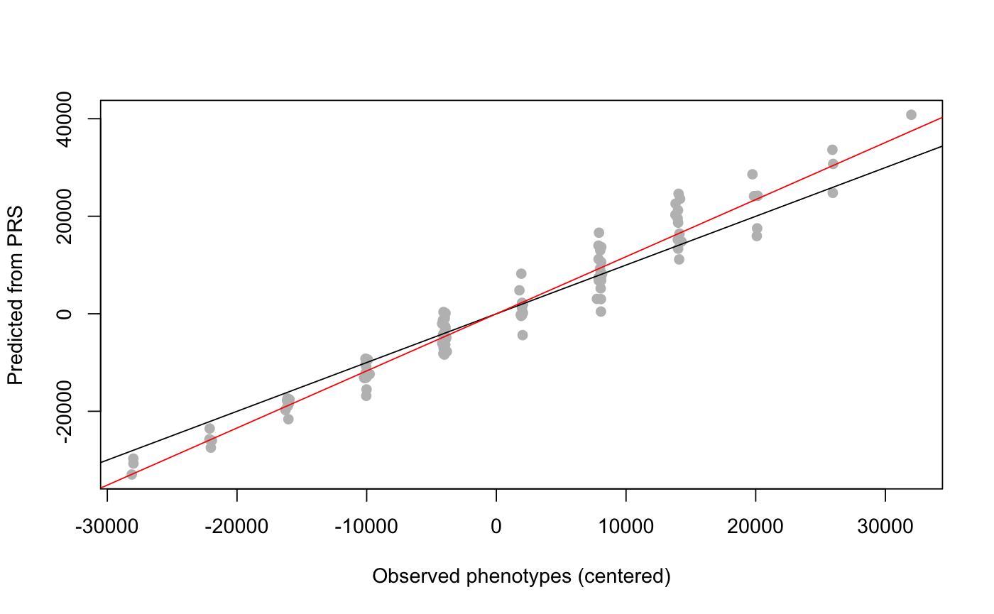
library(lfmm)

## Simulation of 1000 genotypes for 100 individuals (y)
u <- matrix(rnorm(300, sd = 1), nrow = 100, ncol = 2)
v <- matrix(rnorm(3000, sd = 2), nrow = 2, ncol = 1000)
y <- matrix(rbinom(100000, size = 2,
                  prob = 1/(1 + exp(-0.3*(u%*%v
                  + rnorm(100000, sd = 2))))),
                  nrow = 100,
                  ncol = 1000)

#PCA of genotypes, 3 main axes of variation (K = 2) 
plot(prcomp(y))

## Simulation of 1000 phenotypes (x)
## Only the last 10 genotypes have significant effect sizes (b)
b <- matrix(c(rep(0, 990), rep(6000, 10)))
x <- y%*%b + rnorm(100, sd = 100)

## Compute effect sizes using lfmm_ridge
## Note that centering is important (scale = F).
mod.lfmm <- lfmm_ridge(Y = y,
                  X = x,
                  K = 2)

## Compute direct effect sizes using lfmm_ridge estimates
b.estimates <- effect_size(y, x, mod.lfmm)

## plot the last 30 effect sizes (true values are 0 and 6000)
plot(b.estimates[971:1000])
abline(0, 0)
abline(6000, 0, col = 2)

## Prediction of phenotypes
candidates <- 991:1000 #set of causal loci 
x.pred <- scale(y[,candidates], scale = F) %*% matrix(b.estimates[candidates])

## Check predictions
plot(x - mean(x), x.pred,
     pch = 19, col = "grey",
     xlab = "Observed phenotypes (centered)",
     ylab = "Predicted from PRS")
     abline(0,1)
     abline(lm(x.pred ~ scale(x, scale = FALSE)), col = 2)