Analyzing population genomic data with tess3r

Summary: Geography is one of the most important determinant of genetic variation in natural populations. Using genotypic and geographic data, the R package tess3r provides estimates of population genetic structure and tools for screening genomes for signatures of natural selection.

The main function tess3 computes estimates of ancestry proportions and ancestral allele frequencies. The package contains functions that handle geographic maps, and allows users to display spatial representations of ancestry coefficients on those maps. In addition, tess3r performs genome scans for selection by separating adaptive from nonadaptive genetic variation based on allele frequency differentiation tests. Based on matrix factorization algorithms, the tess3r package is parcularly suitable for analyzing large genomic data sets having thousands of markers and samples.

Introduction

Estimating and visualizing population genetic structure is commonly achieved through algorithms such as the well-known STRUCTURE, TESS, ADMIXTURE methods (Pritchard et al. 2000, Chen et al. 2007, Alexander et al. 2009), and with more recent sparse nonnegative matrix factorization approaches (sNMF, Frichot et al. 2014). All these programs estimate proportions of individual genomes originating from K ancestral populations (individual ancestry coefficients), and the corresponding ancestral genotype frequencies.

Population genetic structure analysis includes three main steps:

running one (or more) of the above inference algorithms,
choosing the number of ancestral populations or genetic clusters,
showing bar-plots of ancestry coefficients or displaying them on geographic maps.

This vignette presents a brief tutorial on how to use the R package tess3r to perform all those analyses within a unique framework. The program stores ancestry coefficients in a \(Q\)-matrix, and uses geographic coordinates to visualize results. The algorithm implements a new version of the program TESS (Chen et al. 2007), based on geographically constrained matrix factorization and quadratic programming techniques (Caye et al. 2016). The new algorithms are several order faster than the Monte-Carlo algorithms implemented in previous versions of TESS, and can handle data sets including hundreds of individuals and hundreds of thousands of genotypes. The package can also be used to analyze the input and output files of the Bayesian program TESS 2.3.

The main steps of tess3r are illustrated through the description of two examples. The first example concerns single nucleotide polymorphism (SNP) data for 170 European accessions of the plant species A. thaliana (Atwell et al. 2010). The second example concerns simulated allelic markers (short tandem repeats, STR) for two subspecies hybridizing in Central Europe (Durand et al. 2009).

The next paragraphs will guide users through each step of analysis, making the operations easily reproducible within their computing environment. To start an R session with tess3r, use the following command:

library(tess3r)

SNP data

Data files

Running the main function tess3 requires two files as input to the program: 1) a file encoding individual genotypes, and 2) a file with individual geographic coordinates. Consider SNP data from the plant species A. thaliana in Europe.

data(data.at)
genotype = data.at$X
coordinates = data.at$coord

For SNPs, the genotype matrix encodes individual genotype as rows. Each locus corresponds to a specific column. Genotypes are encoded as 0,1,2 for diploids, and 0,1 for haploids. Those numbers represent the number of reference or derived allele at each particular locus. A. thaliana is a diploid species with very high levels of inbreeding. In our example, 170 genotypes were encoded as haploid (26,943 loci). Let’s print the genotypes for the first 3 individuals at 10 loci. We have a matrix with 0 and 1 values.

dim(genotype)

## [1]   170 26943

genotype[1:3,1:10]

##      [,1] [,2] [,3] [,4] [,5] [,6] [,7] [,8] [,9] [,10]
## [1,]    0    1    1    1    1    1    1    0    1     1
## [2,]    0    1    1    1    1    1    1    0    1     1
## [3,]    0    1    0    1    1    1    1    1    1     1

The genotype file can be read from an external text file having any suffix. The matrix format also corresponds to the .lfmm format in the LEA package (Frichot and Francois, 2015), which contains functions to convert data files from the .ped, .vcf or .geno format into genotypic matrices.

The coordinate file is a two-column file that contains longitude and latitude for each individual in the sample. Longitude (°E) and latitude (°N) must be encoded in the decimal format. Headers must be ignored when loading the data into the R program.

library(maps)
coordinates[1:3,]

##             V1       V2
## [1,] 25.154552 54.39078
## [2,] -8.429345 40.19713
## [3,] 13.511291 55.85332

plot(coordinates, pch = 19, cex = .5, 
     xlab = "Longitude (°E)", ylab = "Latitude (°N)")
map(add = T, interior = F)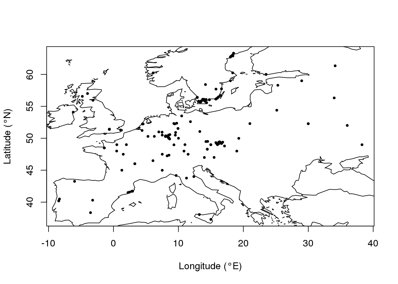

Estimating ancestry coefficients

The main function of the tess3r package is the tess3 function. This function creates an object of class tess3 which contains the results of one or several runs of the estimation algorithm. For example, running the program for ancestral populations numbers ranging from \(K = 1\) to \(K = 8\) using 4 CPUs can be programmed as follows.

tess3.obj <- tess3(X = genotype, coord = coordinates, K = 1:8, 
                   method = "projected.ls", ploidy = 1, openMP.core.num = 4)

The X argument refers to the genotype matrix, the coord argument corresponds to the geographic coordinates, K is the number of clusters or ancestral populations, and openMP.core.num is the number of processes used by the multi-threaded program.

The plot function generates a plot for root mean-squared errors computed on a subset of loci used for cross-validation.

plot(tess3.obj, pch = 19, col = "blue",
     xlab = "Number of ancestral populations",
     ylab = "Cross-validation score")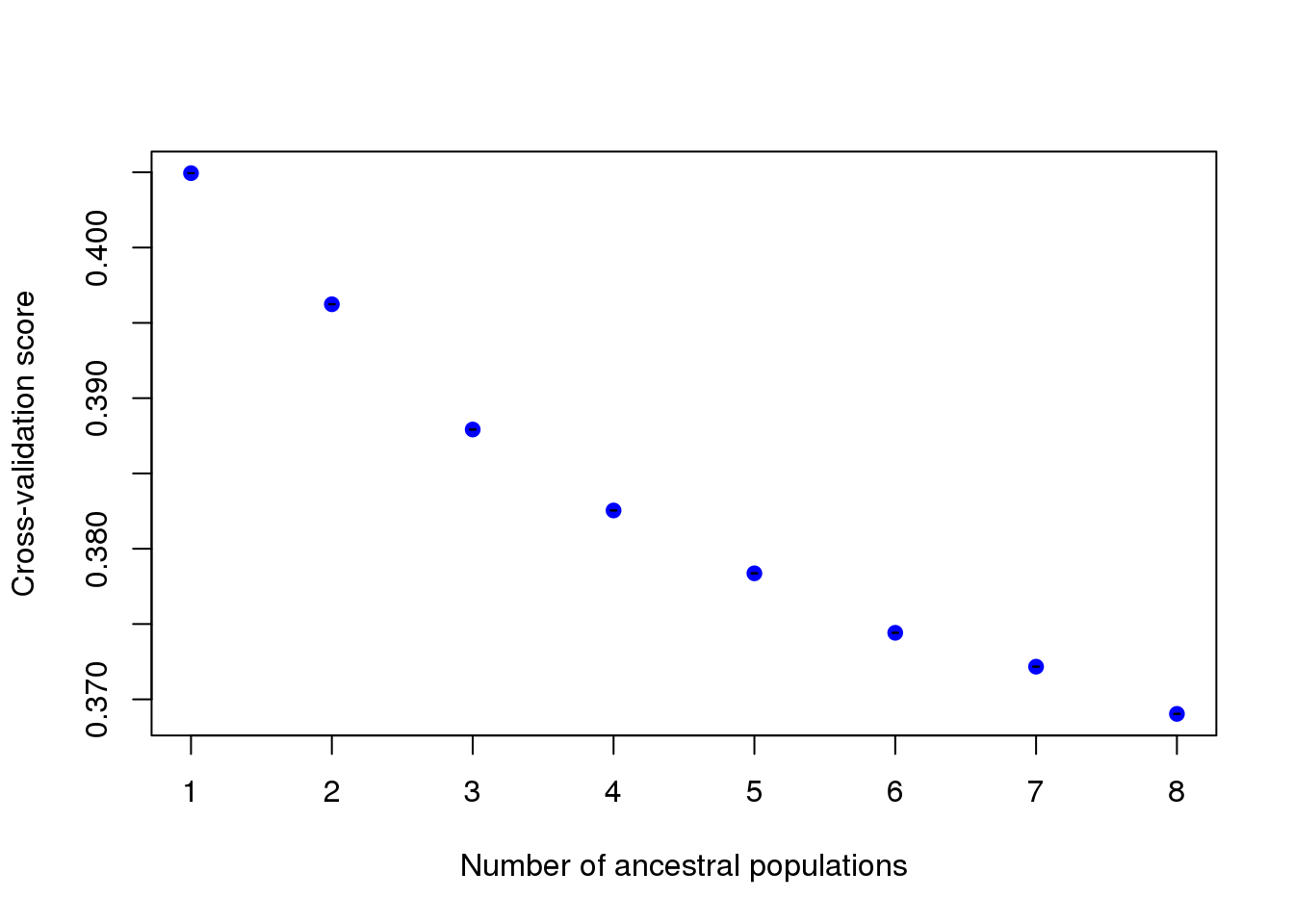

The interpretation of this plot is similar to the cross-entropy plot of LEA or the cross-validation plot of ADMIXTURE. The cross-validation criterion is based on the prediction of a fraction of masked genotypes via matrix completion, and comparison with masked values considered as the truth. Smaller values of the cross-validation criterion mean better runs. The best choice for the \(K\) value is when the cross-validation curve exhibits a plateau or starts increasing.

Warning: Be cautious about over-interpreting the value of \(K\) and the folkore around the choice of this value. Population structure is often hierarchical, and the estimation of \(K\) strongly depends on sampling and genotyping efforts. The number of genetic groups detected by ancestry estimation programs does not necessarily correspond to the number of biologically meaningful populations in the sample (Francois and Durand 2010).

Looking at the results for the A. thaliana data set, the cross-validation criterion does not exhibit a minimum value or a plateau. The result indicates that there are 3 major clusters in Europe, and that finer levels of population structure could be detected.

Visualizing the results

Next, we want to display the \(Q\)-matrix for \(K = 5\) clusters using a barplot representation. For this representation, we use the barplot function of the package.

# retrieve tess3 Q matrix for K = 5 clusters 
q.matrix <- qmatrix(tess3.obj, K = 5)
# STRUCTURE-like barplot for the Q-matrix 
barplot(q.matrix, border = NA, space = 0, 
        xlab = "Individuals", ylab = "Ancestry proportions", 
        main = "Ancestry matrix") -> bp

## Use CreatePalette() to define color palettes.

axis(1, at = 1:nrow(q.matrix), labels = bp$order, las = 3, cex.axis = .4)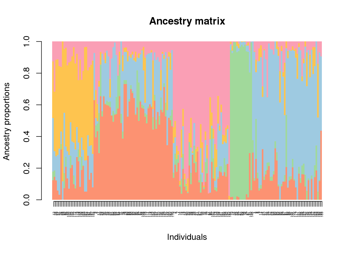

The barplot function is very similar to the default method of the graphics library of R. It contains a ‘sort-by-Q’ option, and allows color palettes to be used. To change the colors, use the CreatePalette function.

my.colors <- c("tomato", "orange", "lightblue", "wheat","olivedrab")
my.palette <- CreatePalette(my.colors, 9)
barplot(q.matrix, border = NA, space = 0, 
        main = "Ancestry matrix", 
        xlab = "Individuals", ylab = "Ancestry proportions", 
        col.palette = my.palette) -> bp
axis(1, at = 1:nrow(q.matrix), labels = bp$order, las = 3, cex.axis = .4)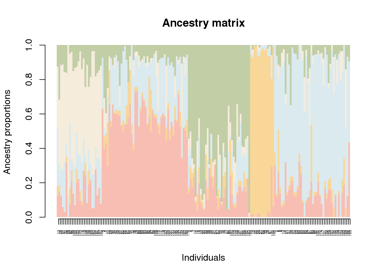

The plot function interpolates the values of the \(Q\)-matrix on a geographic map. The map can be infered from the sample coordinates, or it can be provided to the program in a raster format or a sp::SpatialPolygonsDataFrame object.

plot(q.matrix, coordinates, method = "map.max", interpol = FieldsKrigModel(10),  
     main = "Ancestry coefficients",
     xlab = "Longitude", ylab = "Latitude", 
     resolution = c(300,300), cex = .4, 
     col.palette = my.palette)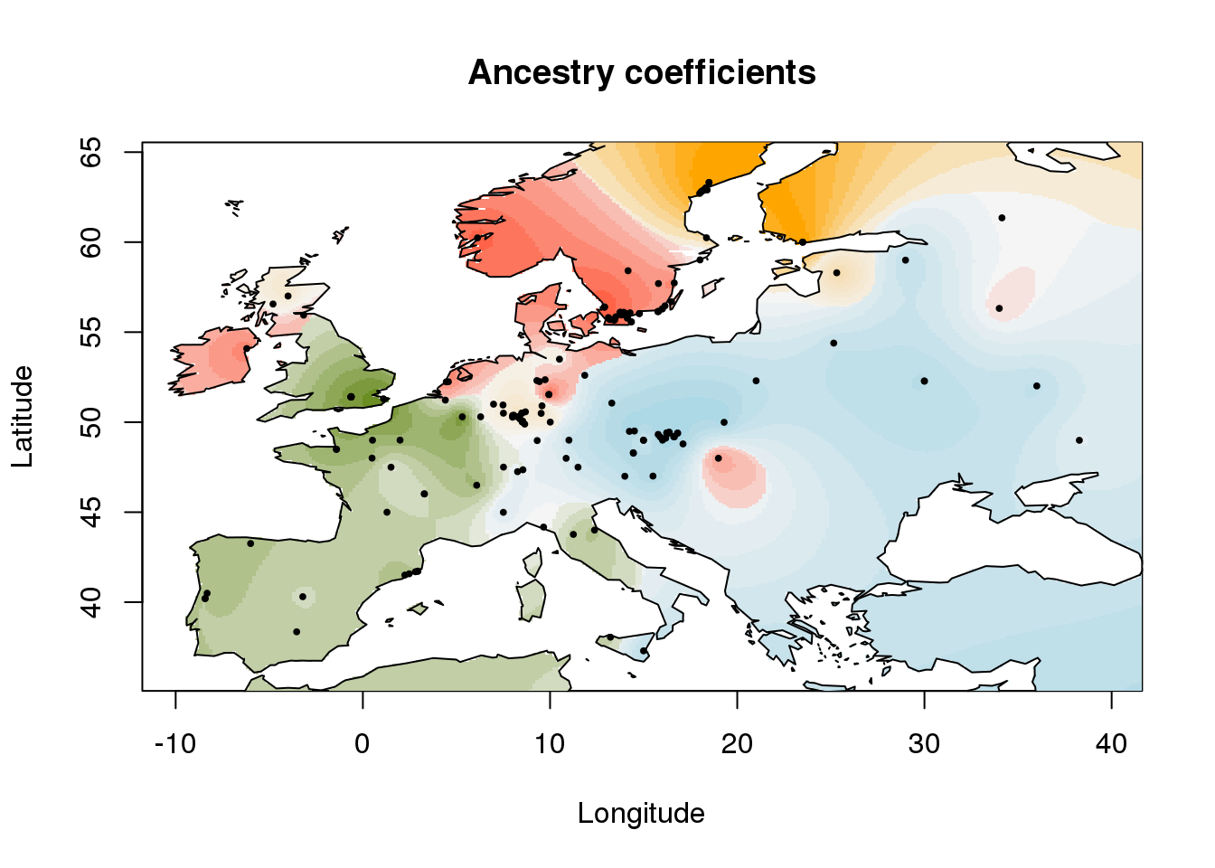

The plot function uses a default world map provide by the function rworldmap::getMap(). For more acurate map, any raster file could be used. For example, a raster map of Europe can be downloaded and used as follows.

asc.raster <- tempfile()
download.file("http://membres-timc.imag.fr/Olivier.Francois/RasterMaps/Europe.asc", asc.raster)
plot(q.matrix, coordinates, method = "map.max", cex = .4,  
     interpol = FieldsKrigModel(10), 
     raster.filename = asc.raster,
     main = "Ancestry coefficients",
     xlab = "Longitude", ylab = "Latitude", 
     col.palette = my.palette)

For ggplot2 enthusiasts, the package provides a function which returns a ggplot layer.

library(ggplot2)
library(rworldmap)

map.polygon <- getMap(resolution = "low")

pl <- ggtess3Q(q.matrix, coordinates, map.polygon = map.polygon)
pl +
  geom_path(data = map.polygon, aes(x = long, y = lat, group = group)) +
  xlim(-16, 42) + 
  ylim(35, 65) + 
  coord_equal() + 
  geom_point(data = as.data.frame(coordinates), aes(x = V1, y = V2), size = 0.2) + 
  xlab("Longitute") +
  ylab("Latitude") + 
  theme_bw()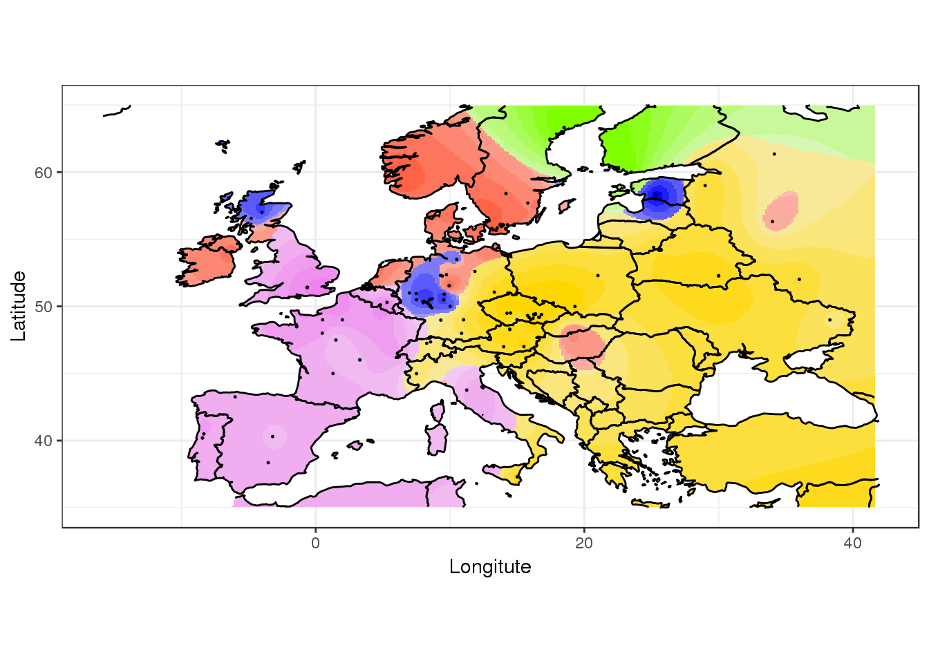

Genome scans for selection

Another feature of the tess3r packages is to allow users to scan the genomic data for outlier loci. The genome scan method implemented in the package is a Fst approach. The function compares single-locus estimates of a population differentiation statistic with the genome-wide background. Then, it converts those estimates into statistical significance values after recalibration of the null-hypothesis (Martins et al. 2016, Francois et al. 2016).

# retrieve tess3 results for K = 5 
p.values <- pvalue(tess3.obj, K = 5)

Whether the tests are correctly calibrated can be checked by inspecting the histogram of \(p\)-values. Ideally, the histogram should be flat and show a peak close to zero.

hist(p.values, col = "lightblue")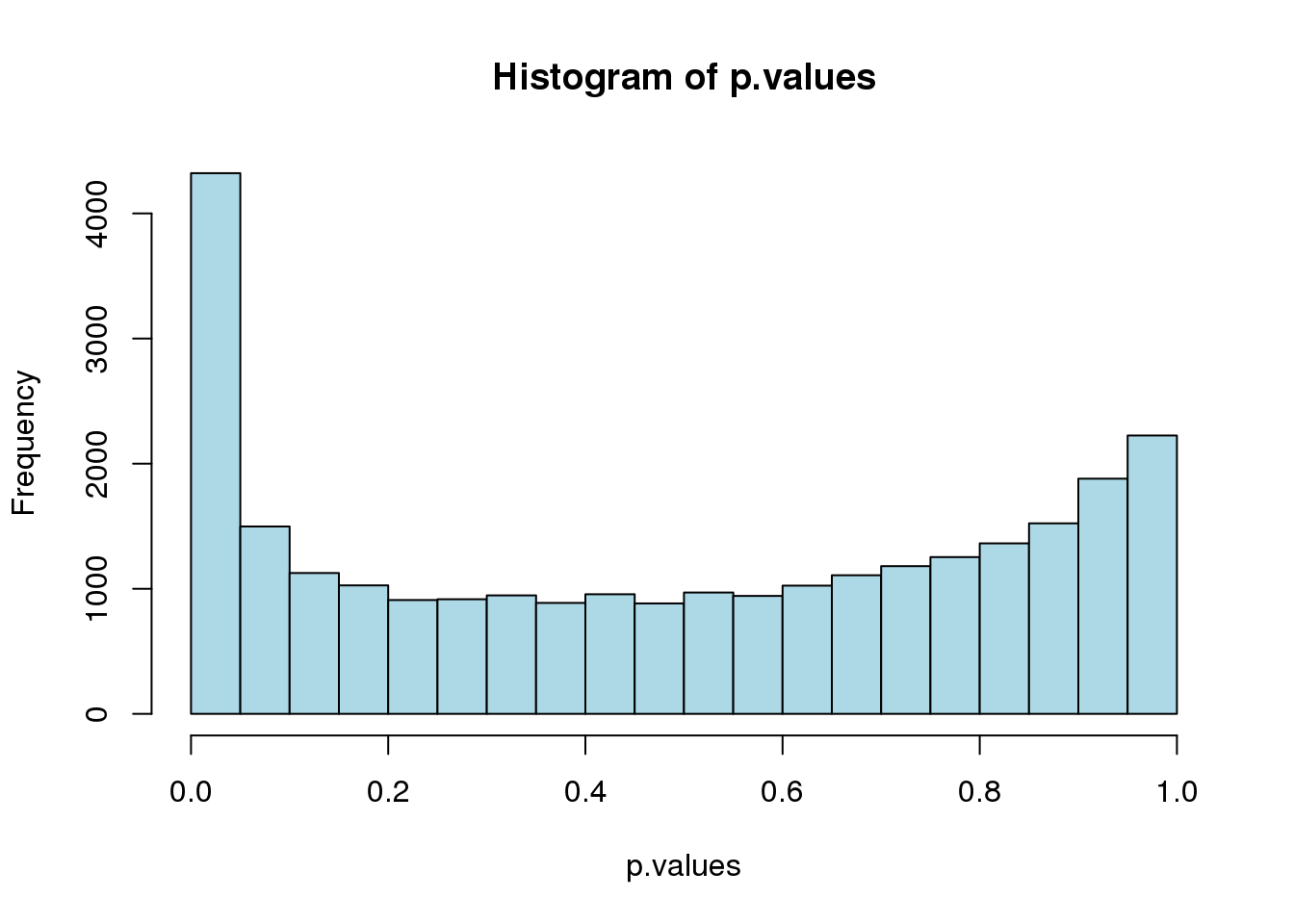

When the histogram has the correct shape, lists of outlier loci can be derived from standard False Discovery Rate (FDR) control algorithms. This can be done by using a classic Benjamini-Hochberg correction as follows.

# Benjamini-Hochberg algorithm
L = length(p.values)
fdr.level = 1e-4
w = which(sort(p.values) < fdr.level * (1:L)/L)
candidates = order(p.values)[w]
length(candidates)

## [1] 433

A list of candidate loci with an expected FDR level of \(0.0001\) is recorded in the object candidates. A ‘Manhattan’ plot highlighting the candidate loci in blue color is then generated as follows.

# manhattan plot 
plot(p.values, main = "Manhattan plot", 
     xlab = "Locus id", 
     ylab = "-log10(P-values)",
     cex = .3, col = "grey")
points(candidates, -log10(p.values)[candidates], 
       pch = 19, cex = .2, col = "blue")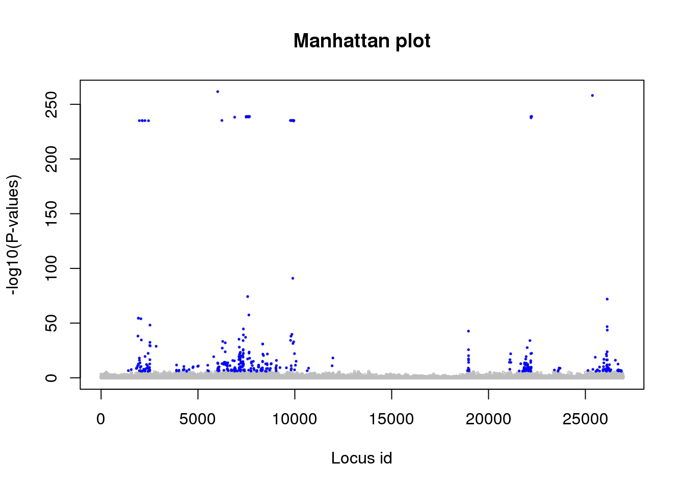

Note that the significance values are displayed on a log scale. The p.values object can also be analyzed with other packages such as the useful qvalue package (Bioconductor).

Multi-allelic data

The tess3r package is not restricted to SNP data sets, and it can provide analyses of population genetic structure for data sets imported from the STRUCTURE or the TESS formats. In this section, we consider an example for simulated microsatellite markers. The data were generated by using a spatially explicit coalescent simulator, and they were analyzed using TESS 2.3 in (Durand et al. 2009).

After an initial phase of divergence, a species started to colonize Europe from two distant southern refugia, one in the Iberian peninsula and the other one in Turkey. Secondary contact occurred in Central Europe, in an area close to Germany. The data consists of 60 population samples of 10 diploid individuals that were genotyped at 100 markers. The data can be loaded and converted as follows.

data(durand09)
d09tess3 <- tess2tess3(durand09, FORMAT = 2, diploid = T, extra.column = 1)

## Input file in the TESS format. The genotypic matrix has 600 individuals and 100 markers. 
## The number of extra rows is 0 and the number of extra columns is 1 .
## The input file contains no missing genotypes.

The tess2tess3 function converts the data in a binary format suitable for tess3, considering each allele as a distinct marker. A boolean value set to TESS = TRUE indicates the TESS format is used (default value). In the TESS format, geographic coordinates (longitude, latitude) are placed at the left to the genotypic matrix. FORMAT is an integer value equal to 1 for markers encoded using one row of data for each individual, and 2 for markers encoded using two rows of data for each individual. Once the file is converted to the binary format, tess3 runs as with the SNP genotypes.

obj.d09 <- tess3(X = d09tess3$X, coord = d09tess3$coord,
             K = 1:10, ploidy = 2, openMP.core.num = 4)
plot(obj.d09, pch = 19, col = "blue",
     xlab = "Number of ancestral populations",
     ylab = "Cross-Validation score")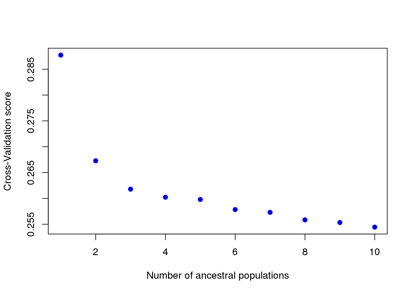

Q.matrix <- qmatrix(obj.d09, K = 3)

The ancestry coefficient matrix can be displayed as follows.

barplot(Q.matrix, sort.by.Q = FALSE, 
        border = NA, space = 0,
        col.palette = my.palette,
        xlab = "Individuals", ylab = "Ancestry coefficients") -> bp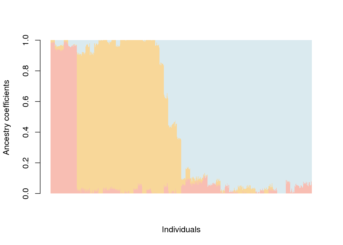

plot(Q.matrix, d09tess3$coord, method = "map.max", cex = .5,  
     interpol = FieldsKrigModel(10), 
     main = "Ancestry coefficients",
     resolution = c(300, 300),
     col.palette = my.palette,
     xlab = "Longitude", ylab = "Latitude")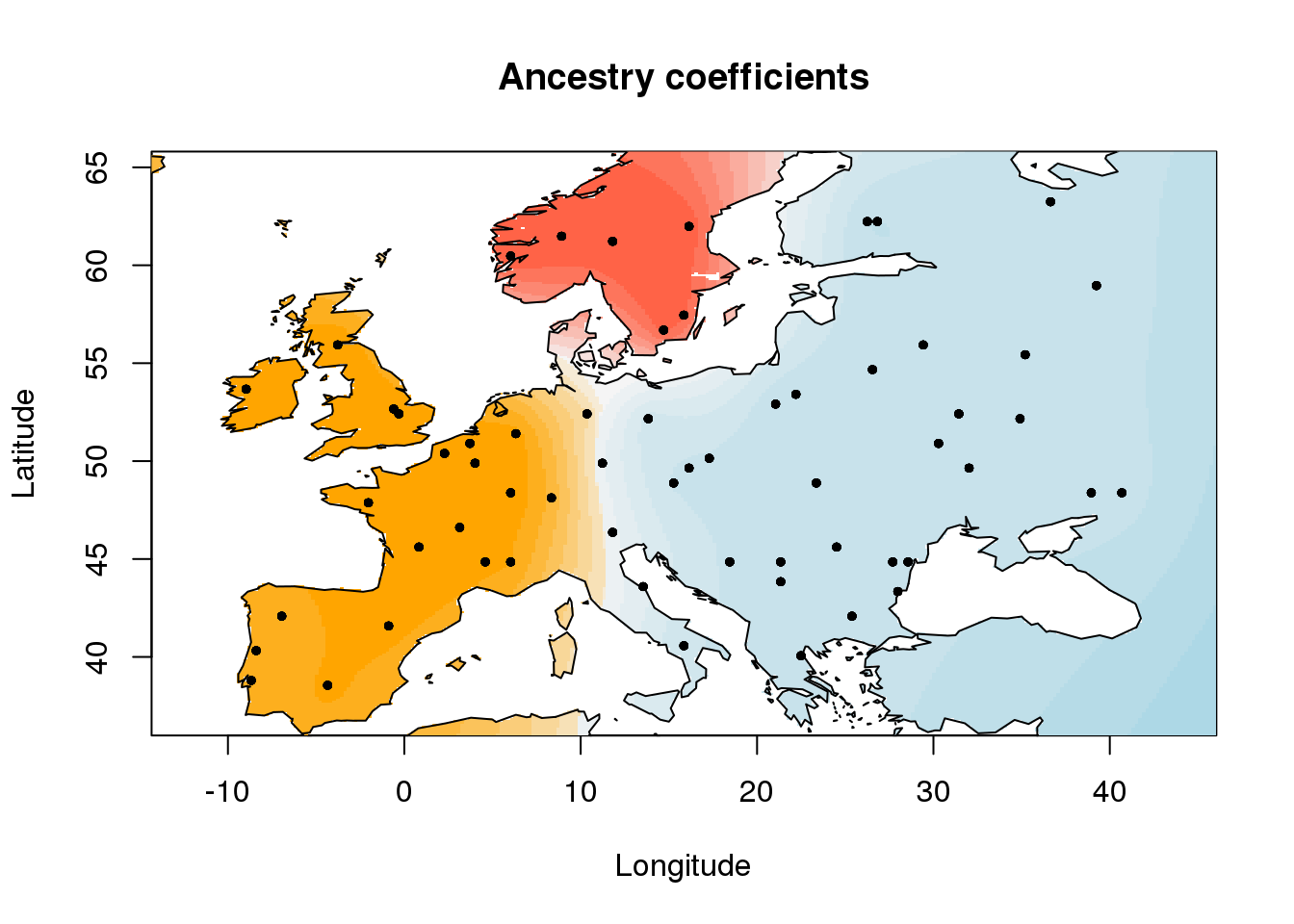

Package reference

Caye K, Jay F, Michel O, Francois O (2016). Fast inference of individual admixture coefficients using geographic data.

References

Alexander DH, Lange K (2011). Enhancements to the ADMIXTURE algorithm for individual ancestry estimation. BMC Bioinformatics 12, 246.
Atwell S, Huang YS, Vilhjalmsson BJ, et al. (2010). Genome-wide association study of 107 phenotypes in Arabidopsis thaliana inbred lines. Nature 465, 627-631.
Caye K, Deist TM, Martins H, Michel O, Francois O (2016). TESS3: Fast inference of spatial population structure and genome scans for selection. Molecular Ecology Resources 16, 540-548.
Chen C, Durand E, Forbes F, Francois O (2007). Bayesian clustering algorithms ascertaining spatial population structure: A new computer program and a comparison study. Molecular Ecology Notes 7, 747-756.
Durand E, Jay F, Gaggiotti OE, Francois O (2009). Spatial inference of admixture proportions and secondary contact zones. Molecular Biology and Evolution 26(9), 1963-1973.
Francois O, Durand E (2010). Spatially explicit Bayesian clustering models in population genetics. Molecular Ecology Resources 10, 773-784.
Francois O, Martins H, Caye K, Schoville SD (2016). Controlling false discoveries in genome scans for selection. Molecular Ecology 25, 454-469.
Frichot E, Francois O (2015). LEA: an R package for Landscape and Ecological Association studies. Methods in Ecology and Evolution 6(8), 925-929.
Frichot E, Mathieu F, Trouillon T, Bouchard G, Francois O (2014). Fast and efficient estimation of individual ancestry coefficients. Genetics 196, 973-983.
Martins H, Caye K, Luu K, Blum MG, Francois O (2016). Identifying outlier loci in admixed and in continuous populations using ancestral population differentiation statistics. Molecular Ecology, (bioRxiv, 054585).
Pritchard JK, Stephens M, Donnelly P (2000). Inference of population structure using multilocus genotype data. Genetics 155(2), 945-959.

Kevin Caye - Flora Jay - Olivier François

2017-07-03