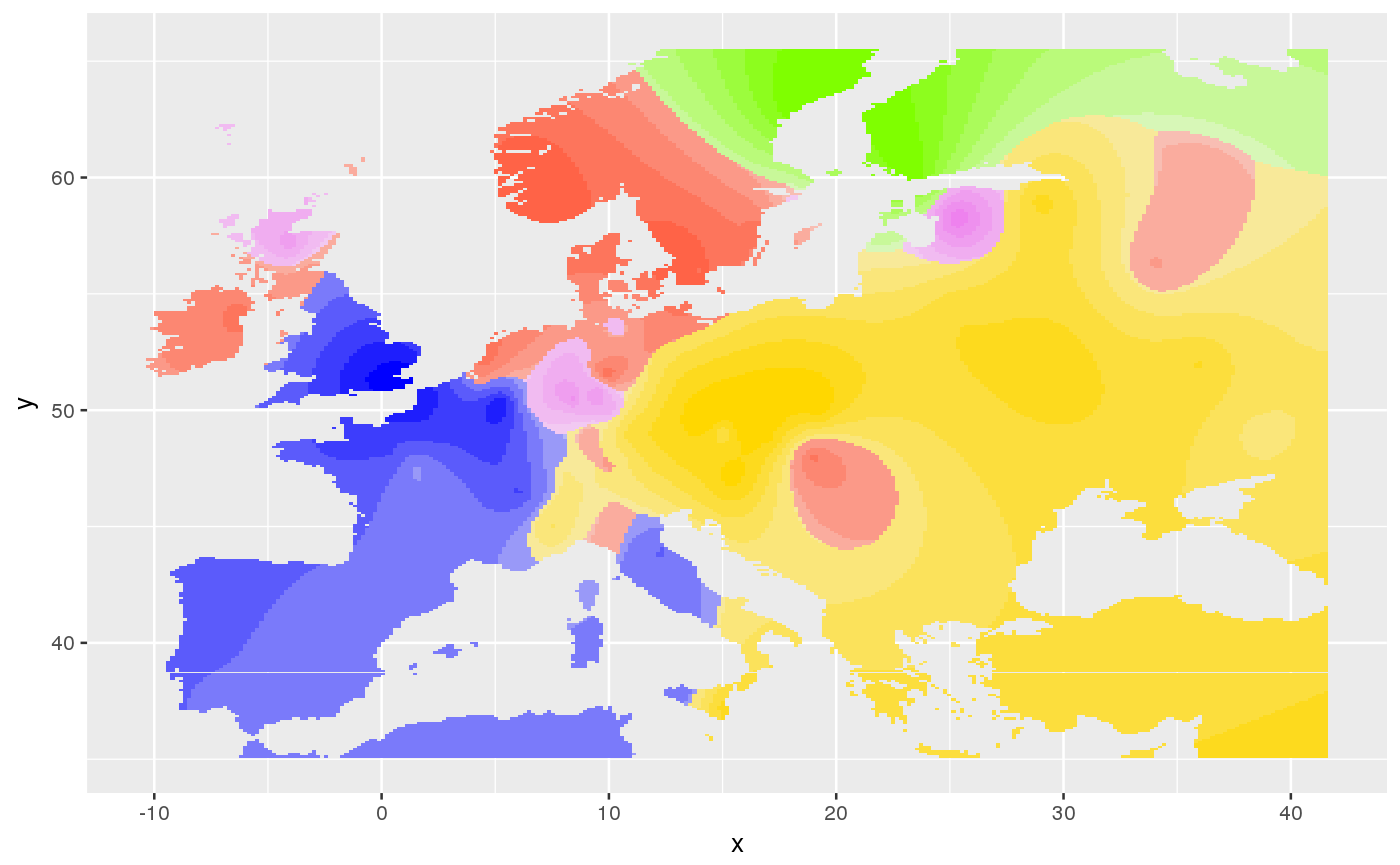
Display geographic maps of ancestry coefficients using the ggplot grammar

This function displays geographic maps of ancestry coefficients using the ggplot syntax.

ggtess3Q(Q, coord, resolution = c(300, 300), window = NULL,
  background = TRUE, map.polygon = NULL, raster.filename = NULL,
  interpolation.model = FieldsKrigModel(10), col.palette = CreatePalette())

Arguments

Q	an object of class tess3Q corresponding to an ancestry coefficient matrix obtained tess3.
coord	a numeric matrix of dimension \(n\) times 2 where \(n\) is the number of individuals. The matrix must contain (Longitude, Latitude) coordinates for all individuals.
resolution	an integer vector resolution = c(rx,ry) for the resolution of the grid used to computed the interpolating surface. rx and ry are resolution numbers for the x-axis and y-axis respectively.
window	an integer vector for the plotting window, such that window = c(xmin, xmax, ymin, ymax) contains the window's min and max coordinates.
background	if TRUE a raster file is used as a stencil to render only raster pixel on earth.
map.polygon	an object of class sp::SpatialPolygonsDataFrame used to crop the interpolating surface. If NULL, the function getMap is used.
raster.filename	a raster file name used to compute the background stencil. This is an alternative method to crop interpolating surfaces. The default method uses map.polygon.
interpolation.model	an interpolation model used to compute the interpolating surface. Interpolation models can use the functions FieldsTpsModel or FieldsKrigModel.
col.palette	a list of color palettes. Color palettes can be defined by using the function CreatePalette.

Value

None

Examples

library(tess3r)

# Load Arabidopsis data
data(data.at)

# Run of TESS3
obj <- tess3(data.at$X, coord = data.at$coord, K = 5,
                 ploidy = 1, method = "projected.ls", openMP.core.num = 4)
#> == Computing spectral decomposition of graph laplacian matrix: done
#> ==Main loop with 4 threads: done

# Get the ancestry matrix
Q.matrix <- qmatrix(obj, K = 5)

# Show a spatial interpolation of the ancestry matrix
ggtess3Q(Q.matrix, data.at$coord)