Estimating cell-type composition accounting for confounder variables.

Based on DNA methylation values, the vignette shows how to estimate cell-type composition and cell type-specific methylation profiles accounting for confounder variables such as age and sex.

Data

We provide access to a simulated matrix D of a complex tissue DNA methylation values. The data frame exp_grp contains the corresponding experimental data for each patient. Here the data frame contains 22 different variables that include sex and age.

D = readRDS(url("https://zenodo.org/record/3247635/files/D.rds"))
dim(D)

## [1] 23381    20

head(D)[1:5, 1:5]

##                  [,1]      [,2]       [,3]      [,4]       [,5]
## cg00000292 0.70429380 1.0000000 0.97145801 1.0000000 0.83341004
## cg00002426 0.09539247 0.2213554 0.06816716 0.0233084 0.09012396
## cg00003994 0.06072960 0.3590995 0.01321180 0.2115948 0.18793080
## cg00005847 0.71071274 1.0000000 1.00000000 1.0000000 1.00000000
## cg00007981 0.00611625 0.0792212 0.02016318 0.3125305 0.01918717

exp_grp = readRDS(url("https://zenodo.org/record/3247635/files/exp_grp.rds"))
dim(exp_grp)

## [1] 20 22

head(exp_grp)[1:5, 1:5]

##      organism       sample_source cigarette_exposure tissue_stage   t
## 1 Homo sapien       Primary Tumor                 NA        adult T1a
## 2 Homo sapien       Primary Tumor                 NA        adult  T2
## 3 Homo sapien       Primary Tumor                 60        adult  T1
## 4 Homo sapien       Primary Tumor                 20        adult T1b
## 5 Homo sapien Solid Tissue Normal                 34        adult T2a

Step 1: removing correlated probes

In addition to cell-type composition, DNA methylation can vary because of other confounder variables, such as age, sex, and batch effects. We use the function CF_detection to remove probes correlated with confounding factors. By default, the function assumes that all variables contained in the argument exp_grp are potential confounders. Using a linear regression for each of the variables, the function removes probes significantly associated with confounders (false discovery threshold defined by the threshold argument).

D_CF = medepir::CF_detection(D, exp_grp, threshold = 0.15, ncores = 2)

dim(D_CF)

## [1] 21487    20

print(paste0("Number of correlated probes removed : ", nrow(D) - nrow(D_CF)))

## [1] "Number of correlated probes removed : 1894"

Step 2: choosing the number of cell types K

To choose the number \(K\) of cell types, we used the function plot_k, which performs a Principal Component Analysis and plot the eigenvalues of the probes matrix in descending order.

medepir::plot_k(D_CF)

To select the number of principal components, we use Cattell rule that recommends to keep principal components that correspond to eigenvalues to the left of the straight line. Here, Cattell rule suggests to keep 4 principal components which corresponds to 5 cell types (the number of cell types is equal to the number of principal components plus one).

Step 3: feature selection

This step is optional. The function feature_selection select probes with the largest variance (5000 probes by default). By removing probes that do not vary, deconvolution routines can run much faster.

D_FS = medepir::feature_selection(D_CF)

dim(D_FS)

## [1] 4999   20

Step 4: running deconvolution methods

We propose three methods of deconvolution, of three packages: RFE to run RefFreeEWAS::RefFreeCellMix, MDC to run MeDeCom::runMeDeCom and Edec to run EDec::run_edec_stage_1.

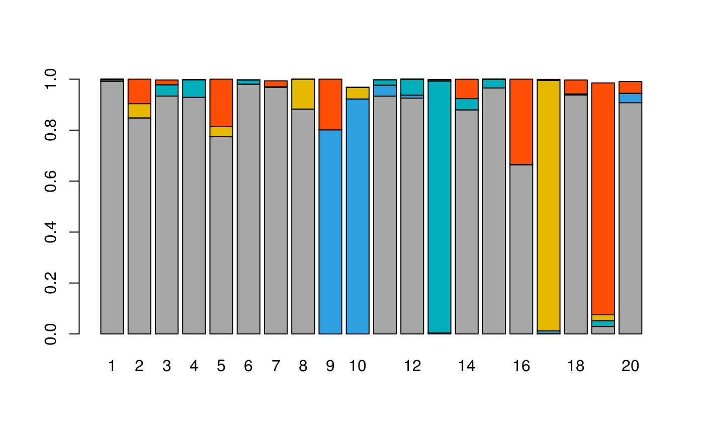
Here we show the results obtained with RefFreeEWAS.

results_RFE = medepir::RFE(D_FS, nbcell = 5)

## The "ward" method has been renamed to "ward.D"; note new "ward.D2"

##      Min.   1st Qu.    Median      Mean   3rd Qu.      Max. 
## 4.600e-07 2.266e-03 5.265e-03 8.524e-03 1.110e-02 8.599e-02 
##     Min.  1st Qu.   Median     Mean  3rd Qu.     Max. 
## 0.000000 0.001734 0.003882 0.006065 0.007735 0.061033 
##     Min.  1st Qu.   Median     Mean  3rd Qu.     Max. 
## 0.000000 0.001343 0.003002 0.004482 0.005753 0.043014 
##     Min.  1st Qu.   Median     Mean  3rd Qu.     Max. 
## 0.000000 0.001088 0.002383 0.003300 0.004391 0.028942 
##     Min.  1st Qu.   Median     Mean  3rd Qu.     Max. 
## 0.000000 0.000873 0.001899 0.002490 0.003440 0.019102 
##      Min.   1st Qu.    Median      Mean   3rd Qu.      Max. 
## 0.0000000 0.0007163 0.0015768 0.0020071 0.0028159 0.0136193 
##      Min.   1st Qu.    Median      Mean   3rd Qu.      Max. 
## 0.0000000 0.0006118 0.0013481 0.0016938 0.0023925 0.0106228 
##      Min.   1st Qu.    Median      Mean   3rd Qu.      Max. 
## 0.0000000 0.0005413 0.0011860 0.0014716 0.0020968 0.0083315 
##      Min.   1st Qu.    Median      Mean   3rd Qu.      Max. 
## 0.0000000 0.0004882 0.0010600 0.0013014 0.0018606 0.0069595

Results obtained with EDec and MeDeCom can be obtained by uncommenting the following code.

#results_MDC = medepir::MDC(D_FS, nbcell = 5, lambdas = c(0, 10^(-5:-1)))

#infloci = read.table(url("https://zenodo.org/record/3247635/files/inf_loci.txt"),header = FALSE, sep = "\t")
#infloci = as.vector(infloci$V1)
#results_Edec = medepir::Edec(D, nbcell = 5, infloci = infloci)

Step 5: vizualizing results

We can vizualize the matrix of cell-type proportions using a stacked bar plot.

proportions<-(results_RFE$A)
colors <- c("#A7A7A7","#2E9FDF", "#00AFBB", "#E7B800", "#FC4E07")
barplot(proportions,names.arg=1:20,col=colors)

Michael Blum, Clémentine Decamps, Florian Privé, Magali Richard